Timeseries
Time series forecasting enables you to predict future values based on historical data, making it invaluable for tasks such as stock price prediction, demand forecasting, and more. This section outlines the key configurations and settings for building time series models on the EvoML platform.
For a step-by-step guide on creating a time series trial, refer to this tutorial.
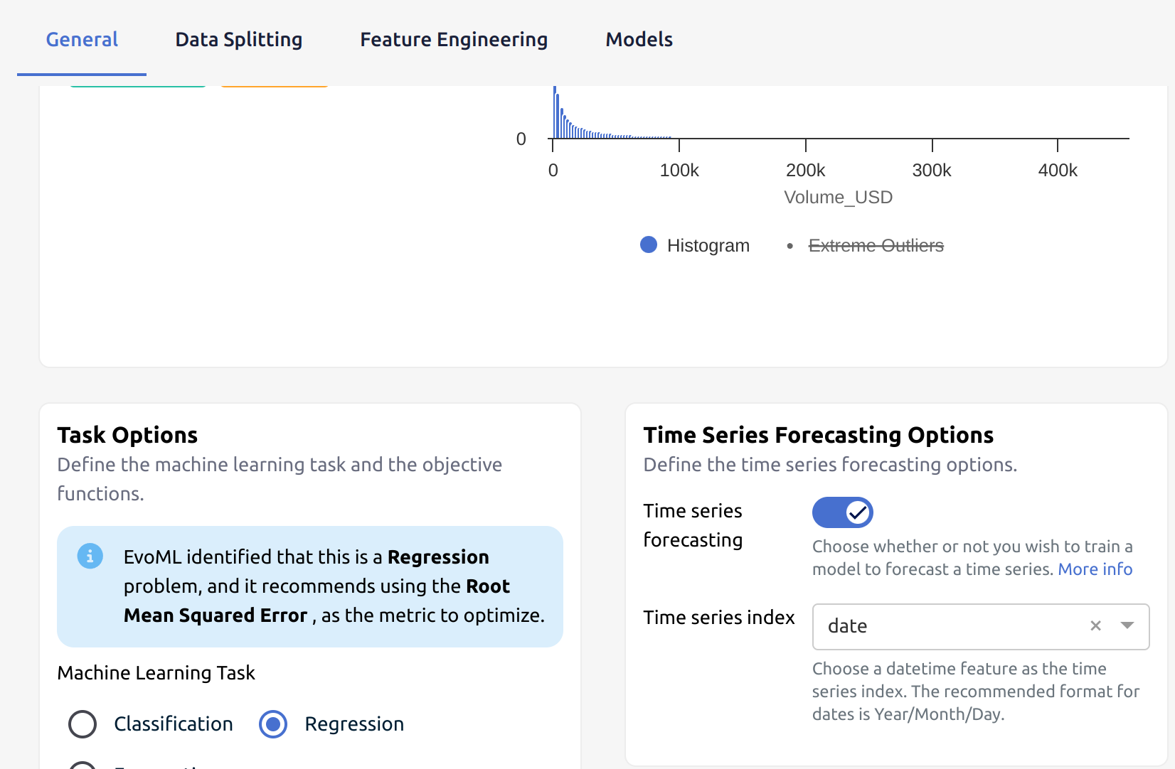
1. Enable Time Series
To start a time series trial on EvoML:
-
Create a New Trial: Begin by creating a new trial in the EvoML platform.
-
Enable Time Series Forecasting: Select the option to enable time series forecasting for your trial.
-
Select Time Series Index: Choose the time component of your data (e.g., a column with timestamps or date values) that will be used to define the sequence. This column serves as the index for temporal ordering.
2. Model Validation
Time series forecasting requires specific validation methods to ensure that the temporal order of the data is preserved. These methods prevent data leakage and ensure the model is tested correctly.
To access Model validation:
- Create New Trial
- Navigate to Data Splitting tab and choose Model Validation
Unlike standard cross-validation, time series models use the following validation methods, which account for temporal dependencies:
- Holdout: A simple approach where a portion of the data is set aside for validation, without shuffling.
- Sliding Window Validation: The training set is moved forward in time to validate across multiple windows, ensuring the model is evaluated over different time segments.
- Expanding Window Validation: The training set grows as new data points are added, helping evaluate the model’s ability to generalize over time.
These methods ensure no future data points are used to predict past values, thus preventing information leakage. Further details on model validation can be found here.
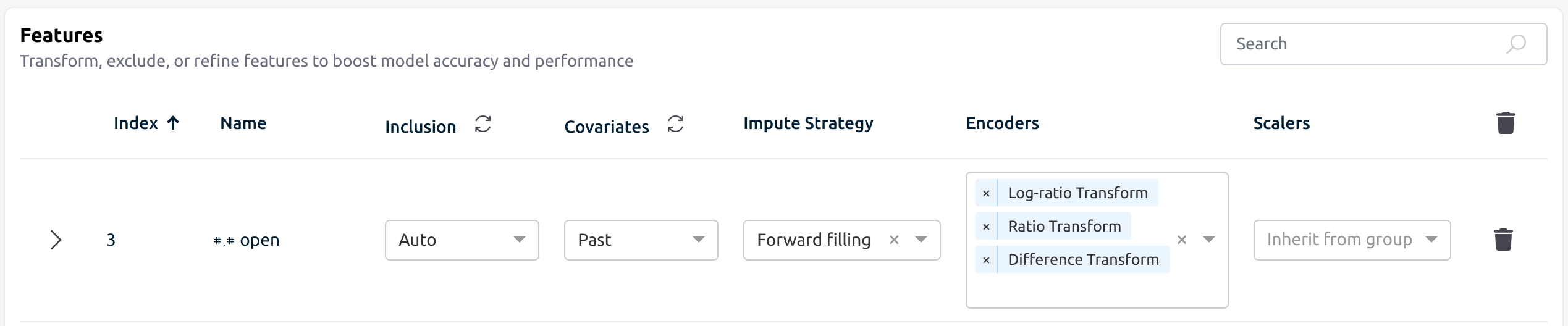
3. Feature Options
EvoML provides several strategies to handle missing values, encode trends, and scale your time series data. The platform includes time series-specific options as described below.
Impute Strategies
Time series often contain missing values. The following strategies are available to impute or fill in these gaps:
- Forward Filling: Fills missing values with the last observed value, propagating it forward.
- Backward Filling: Fills missing values with the next valid observation, though use cautiously to avoid data leakage.
- Linear Interpolation: Fills missing values by estimating a straight line between the surrounding data points.
- Spline Interpolation: Uses a smooth curve to estimate missing values, providing a more accurate fit than linear methods.
- Moving Average: Fills gaps using the mean of surrounding values, calculated over a rolling window.
- Polynomial Interpolation: Uses higher-order polynomials to estimate missing values, which can offer more precision than linear methods.
Encode Strategies
To reveal trends and relationships in your data, EvoML offers the following encoding strategies:
- Difference Transform: Computes the difference between values separated by the forecast horizon, highlighting trends and seasonality.
- Ratio Transform: Calculates the ratio between values separated by the forecast horizon, helping normalize fluctuating data and identify growth patterns.
- Log-Ratio Transform: Applies a logarithmic transformation to the ratio between values, stabilizing variance and normalizing the data.
4. Feature Engineering
EvoML automatically performs feature engineering for time series data by generating lagged features. These features are created by shifting historical values of a variable by a specified number of time steps. This allows the model to capture temporal dependencies and patterns.
When using regression or classification models to forecast, you must specify:
- Which features are past or future covariates.
- The context window (the number of past-time steps the model will consider).
- The forecast horizon (the number of future time steps the model will predict).
Below is an example screenshot that shows how to configure covariates, set the context window, and define the forecast horizon:
Covariates in Forecasting
In time series forecasting, covariates are additional features that can be used to improve model predictions. Covariates can be categorized into:
- Past Covariates: Variables that are only known after the timestamp they correspond to (e.g., sales data for a specific day, only known once the day is over).
- Future Covariates: Variables that are known ahead of time (e.g., whether a given day will fall on a weekend).
Context Window
The Context Window defines how many previous time steps are considered for predicting future values. This determines how far back in time the model looks during training and forecasting.
Example: If you set a context window of 5 months, the model will use data from the last 5 months to make predictions about future values.
Forecast Horizon
The Forecast Horizon specifies how many time steps ahead the model will predict. It represents the length of the forecast period, which can be customized based on your needs.
Example: With a forecast horizon of 7 days, the model will predict values for the next 7 days based on the historical data within the context window.