US Unemployment

Overview

This notebook aims to build and query a model to forecast the US unemployment rate. Along the way,we will demonstrate how the evoML Python Client facilitates integration with external sources. In this case, we will use the Federal Reserve Bank (FRED) API (https://fred.stlouisfed.org/docs/api/fred) to retrieve various macroeconomic timeseries, joining them and upload them to the evoML platform to begin a trial.

This notebook can also be viewed at https://nbviewer.org/url/docs.evoml.ai/notebooks/forecasting-unemployment.ipynb.

Setup

Dependencies

This notebook uses the following library versions:

• turintech-evoml-client
• fredapi
• pandas
• matplotlib

Credentials

You will also require:

• A URL for an instance of the evoML platform (e.g. https://evoml.ai)
• Your evoML username and password
• An API key for the Federal Reserve Bank (FRED). A free key can be obtained at: https://fred.stlouisfed.org/docs/api/api_key.html

import pandas as pd
import matplotlib.pyplot as plt
from typing import Final
from fredapi import Fred

import evoml_client as ec
from evoml_client.trial_conf_models import BudgetMode, SplitMethodOptions


# Set credentials and API key
API_URL: Final[str] = "https://evoml.ai"
EVOML_USERNAME: Final[str] = ""
EVOML_PASSWORD: Final[str] = ""
FRED_API_KEY: Final[str] = ""

# Connect to the evoML platform
ec.init(base_url=API_URL, username=EVOML_USERNAME, password=EVOML_PASSWORD)

# Initialize the FRED API client
fred = Fred(api_key=FRED_API_KEY)

Data Preparation

We will first need to retrieve some data to predict the unemployment rate. The symbol for the unemployment rate is UNRATE (https://fred.stlouisfed.org/series/UNRATE), but we will also retrieve the gross domestic product GDP (https://fred.stlouisfed.org/series/GDP), and leading economic index USSLIND (https://fred.stlouisfed.org/series/USSLIND).

These datasets are sampled at different frequencies and cover different time periods so, after the download is complete, we will join them and resample to monthly frequency before uploading the final dataset to the platform.

# Download data from FRED
symbols = ['UNRATE', 'USSLIND', 'GDP']
data_dict = {symbol: fred.get_series(symbol) for symbol in symbols}

# Join datasets
data_fred = pd.concat(data_dict.values(), axis=1)
data_fred.columns = symbols

# Resample to monthly frequency
data_fred = data_fred.resample('M').mean()

# Use data since 1950
data_fred = data_fred.loc[pd.Timestamp('1950-01-01'):]

# Reset the index as a column
data_fred.reset_index(inplace=True)

# Upload and wait for completion of task
dataset = ec.Dataset.from_pandas(data_fred, name="Economic Indicators")
dataset.put()
dataset.wait()
print(f"Dataset URL: {API_URL}/platform/datasets/view/{dataset.dataset_id}")

Running a Trial

Once your dataset is uploaded, you can run a trial to generate and evaluate models. In this example, we use the Mean Absolute Error (MAE) as the loss function because it is simple to interpret and robust to outliers. The timeSeriesWindowSize is set to 6, meaning the model will use data from the last 6 months to make predictions. The timeSeriesHorizon is set to 12, indicating that we aim to forecast 12 months into the future. A typical trial configuration looks like this:

train_percentage = 0.8
config = ec.TrialConfig.with_models(
    models=["linear_regressor", "elastic_net_regressor", "ridge_regressor", "bayesian_ridge_regressor"],
    task=ec.MlTask.regression,
    budget_mode=BudgetMode.fast,
    loss_funcs=["Mean Absolute Error"],
    dataset_id=dataset.dataset_id,
    is_timeseries=True,
)
config.options.timeSeriesWindowSize = 6
config.options.timeSeriesHorizon = 12
config.options.splittingMethodOptions = SplitMethodOptions(method="percentage", trainPercentage=train_percentage)
config.options.enableBudgetTuning = False

trial, _ = ec.Trial.from_dataset_id(
    dataset.dataset_id,
    target_col="UNRATE",
    trial_name="Forecast - Unemployment Rate",
    config=config,
)

trial.run(timeout=900)

Interacting with Pipelines

Building the Pipeline

After a trial is completed, we can retrieve and use the best pipeline for predictions. Here we demonstrate how to use the pipeline to make online predictions, meaning the model is deployed inside the evoML platform and can be queried for new predictions.

# Retrieve the top ranked pipeline on the objective function
pipeline = trial.get_best()

# Online prediction
data_online = pipeline.predict_online(dataset=dataset)

After a couple of minutes the platform will complete the build and deployment of the model and finish the predictdions. We can now retrieve the metrics calculated during the trial and visualise the results.

# Retrieve the mean absolute error (MAE) for train, validation, and test sets found during the build-model
mae_train = pipeline.model_rep.metrics["regression-mae"]["train"]["average"]
mae_validation = pipeline.model_rep.metrics["regression-mae"]["validation"]["average"]
mae_test = pipeline.model_rep.metrics["regression-mae"]["test"]["average"]
print(f"Mean Absolute Error (MAE) on Train Set: {mae_train}")
print(f"Mean Absolute Error (MAE) on Validation Set: {mae_validation}")
print(f"Mean Absolute Error (MAE) on Test Set: {mae_test}")

We find the metrics from the trial are as follows:

Split	Mean Absolute Error (MAE)
Train	0.737
Validation	0.668
Test	0.926

Visualising Predictions

Finally we plot predictions from our pipeline over the entire range of training and testing data. The test range is shaded on the right hand side.

plt.figure(figsize=(15, 6))
plt.plot(data_online["index"], data_online["UNRATE"], label="Actual")
plt.plot(data_online["index"], data_online["Prediction"], label="Predicted", linestyle='--')

# Calculate the index where the test range starts
train_end_index = int(len(data_online) * train_percentage)
test_start_date = data_online["index"].iloc[train_end_index + 1]

# Add shaded block for the test range
plt.axvspan(test_start_date, data_online["index"].max(), color='gray', alpha=0.3, label='Test Range')
plt.xlim(data_online["index"].min(), data_online["index"].max())

plt.xlabel("Date")
plt.ylabel("UNRATE")
plt.title("Actual vs Predicted UNRATE")
plt.legend()
plt.show()

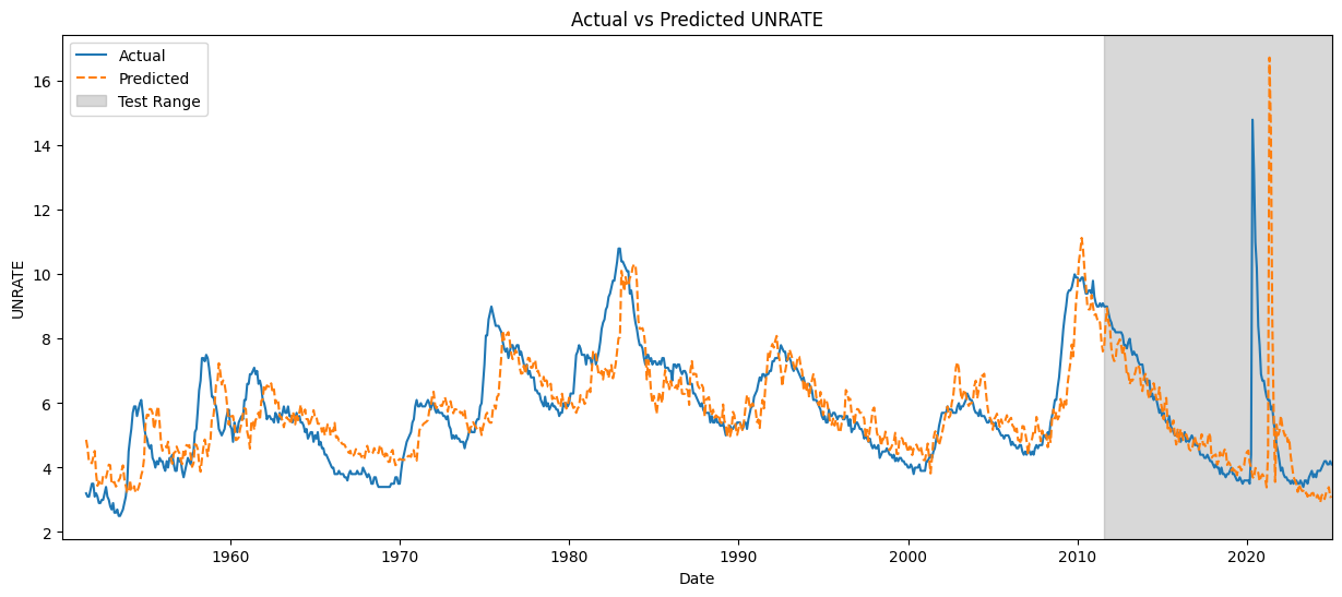
In the test range, the model closely follows actual values before COVID-19, showing strong predictive accuracy under normal conditions. However, during the onset of COVID-19, the model fails to capture the sharp spike in unemployment, likely due to the unprecedented nature of the event and the lack of similar disruptions in the training data.