Household Power Consumption

Overview

In this notebook, we will give an example of how you can use evoML to build a predictive model for future daily household power consumption. We will be using the daily cumulative power consumptions of 955 households in Germany over a period from November 2017 to October 2020. In this example we will be forecasting the mean household.

This notebook can also be viewed at https://nbviewer.org/url/docs.evoml.ai/notebooks/predicting-power-consumption.ipynb.

Setup

Dependencies

This notebook uses the following dependencies:

• turintech-evoml-client
• pandas
• matplotlib

Credentials and Dataset

You will also require:

• A URL for an instance of the evoML platform (e.g. https://evoml.ai).
• Your evoML username and password.
• After creating an IEEE account the all-users-daily-data.csv dataset is freely available at: https://ieee-dataport.org/open-access/gem-house-opendata-german-electricity-consumption-many-households-over-three-years-2018.

import pandas as pd
import matplotlib.pyplot as plt
from typing import Final

import evoml_client as ec
from evoml_client.trial_conf_models import BudgetMode

# Load credentials from environment variables
API_URL: Final[str] = "https://evoml.ai"
EVOML_USERNAME: Final[str] = ""
EVOML_PASSWORD: Final[str] = ""

# Connect to the evoML platform
ec.init(base_url=API_URL, username=EVOML_USERNAME, password=EVOML_PASSWORD)

Data Preparation

Mean Daily Energy Consumption

After downloading the all-users-daily-data.csv dataset, we will load it into a pandas DataFrame and convert the raw meter readings to kilowatt-hours (kWh). We will then calculate the daily power consumption of each household and resample the data to ensure daily frequency. The data is stored in a narrow format and the households are distinguished by the userId column.

cumulative_energy = pd.read_csv("all-users-daily-data.csv")
cumulative_energy["energy"] *= 1e-10  # Convert from raw meter readings to kWh

# Function to standardize time index and compute daily energy
def calculate_daily_energy(df):
    return (
        df.assign(date=pd.to_datetime(df['date'])) # Ensure date column is in datetime format
        .set_index('date')                         # Set date column as the index
        .resample('D')                             # Resample to ensure daily frequency
        .asfreq()                                  # Fill missing dates with NaNs
        .assign(daily_energy=lambda x: x['energy'].diff())  # Compute daily energy difference
    )

# Apply the function groupwise and standardize the time index
daily_energy = cumulative_energy.groupby('userId').apply(calculate_daily_energy)

# Group by date and calculate the mean daily_energy
mean_daily_energy = daily_energy.pivot_table(values='daily_energy', index='date', aggfunc='mean')

Exploratory Data Analysis

To get some idea of what's going on in our data we will now visualize the mean daily power consumption.

mean_daily_energy["daily_energy"].plot(figsize=(15, 6), linestyle='-')
plt.title('Mean Daily Energy Consumption Across All Users Over Time')
plt.xlabel('Date')
plt.ylabel('Mean Daily Energy Consumption')
plt.xticks(rotation=45)
plt.grid(True)
plt.show()

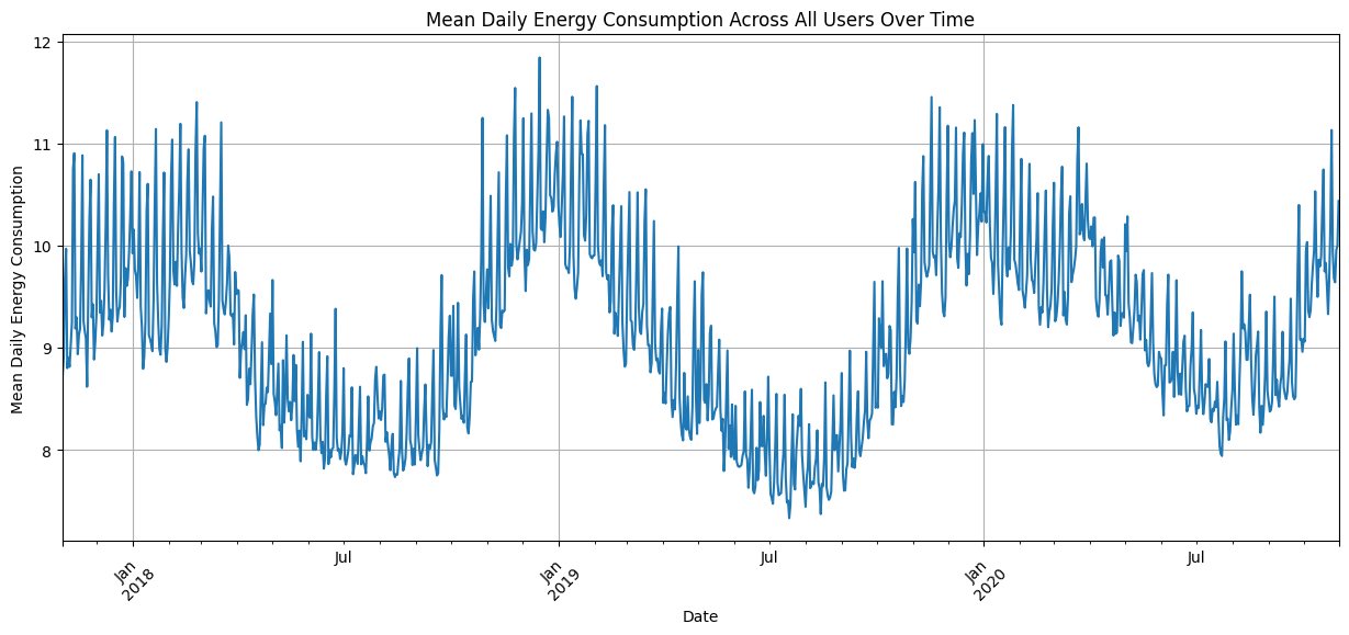
Immediately we can see that the daily power consumption follows a slow yearly cycle with the addition of a lower amplitude weekly cycle. This will be useful when setting up a trial.

Upload to evoML

In order to prepare a trial, we first need to upload a dataset. We will perform this task from within the current notebook using the evoML client.

# Upload the dataset
dataset = ec.Dataset.from_pandas(mean_daily_energy.reset_index(), name="Mean Daily Energy Consumption")
dataset.put()
dataset.wait()
print(f"Dataset URL: {API_URL}/platform/datasets/view/{dataset.dataset_id}")

Running a Trial

With our dataset loaded, we can now set up a trial to predict the daily power consumption of each household. We first create a configuration, before creating a trial object and running it.

config = ec.TrialConfig.with_default(
    task=ec.MlTask.regression,
    budget_mode=BudgetMode.fast,
    loss_funcs=["R2"],
    dataset_id=dataset.dataset_id,
    is_timeseries=True,
)
config.options.timeSeriesWindowSize = 7
config.options.enableBudgetTuning = False

trial, dataset = ec.Trial.from_dataset_id(
    dataset.dataset_id,
    target_col="daily_energy",
    trial_name="Forecast - Daily Energy",
    config=config,
)

trial.run(timeout=900)

metrics = trial.get_metrics_dataframe()
selected_metrics = metrics.loc[:, pd.IndexSlice["regression-r2", ["validation", "test"]]]
selected_metrics.sort_values(by=("regression-r2", "validation"), ascending=False)

Model	Validation R2	Test R2
linear_regressor-7dc3d	0.845	0.817
lightgbm_regressor-424fa	0.834	0.831
decision_tree_regressor-5a883	0.761	-0.787

We see that on the validation set the best model was a linear model which achieved an R2 score of 0.845. Let's get the pipeline for this model and use it to predict the daily power consumption of the last 4 weeks of data.

Interacting with Pipelines

Building the Pipeline

After a trial is completed, we can retrieve and use the best pipeline for predictions. Here we demonstrate how to use the pipeline to make online predictions.

# Retrieve the best model according to the specified objective function and validation set
best_model = trial.get_best()

# Build the model so that we can use it for prediction
best_model.build_model()

Visualizing Predictions

Now we create the test set for prediction and visualization and plot the results.

# Select n_days of data
n_days = 7*4
test_data = mean_daily_energy.iloc[-n_days:]

# Predict the mean daily energy
predicted_mean_daily_energy = pd.Series(best_model.predict(data=test_data.reset_index()), index=test_data.index)

# Plot the actual and predicted mean daily energy without auto-legend
ax = test_data.plot(
    figsize=(15, 6),
    linestyle='-',
    label='Actual',
    legend=False
)
predicted_mean_daily_energy.plot(
    ax=ax,
    linestyle='--',
    label='Predicted',
    legend=False
)
ax.legend(['Actual', 'Predicted'])

plt.title('Mean Daily Energy Consumption: Actual vs Predicted')
plt.xlabel('Date')
plt.ylabel('Mean Daily Energy Consumption')
plt.xticks(rotation=45)
plt.grid(True)
plt.show()

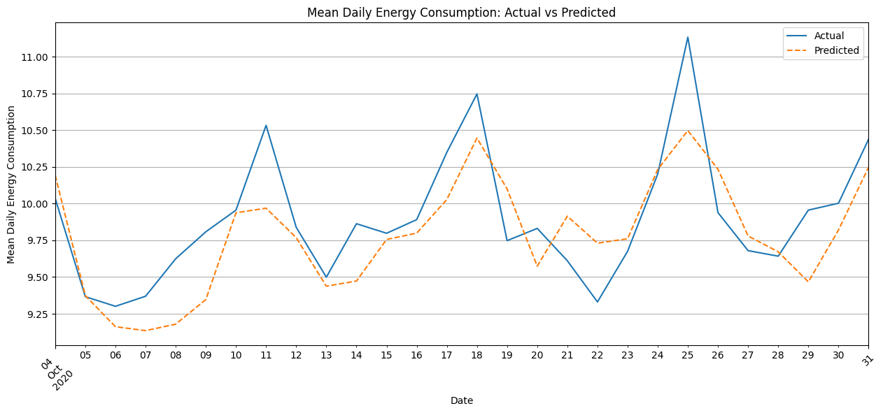
The predicted values generally align with the trend of actual energy consumption but do not fully capture sharp peaks and troughs, such as those around the 11th, 19th, and 25th. This suggests the model smooths the predictions and has limited sensitivity to sudden daily variability.