Regression Metrics

Regression metrics evaluate the performance of a regression model. The following metrics provide different insights into model accuracy, error magnitude, and predictive reliability. Selecting the right metric depends on the problem's specifics, such as sensitivity to large errors, need for explainability, and computational efficiency.

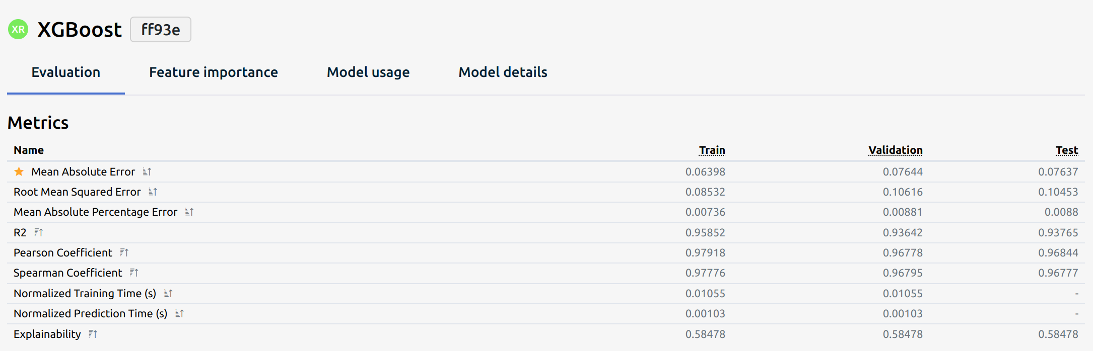
Each regression model is evaluated using these metrics:

---

1. Mean Absolute Error (MAE)

Definition: MAE measures the average absolute differences between predicted and actual values. Lower values indicate better performance.

$$\text{MAE} = \frac{1}{N} \sum_{i=1}^{N} | y_i - \hat{y}_i |$$

Where:

• ($y_i$) = actual value
• ($\hat{y}_i$) = predicted value
• ($N$) = number of observations

Use Case: Useful when all errors should be treated equally, regardless of direction.

---

2. Root Mean Squared Error (RMSE)

Definition: RMSE calculates the square root of the average squared errors, penalizing larger errors more heavily.

$$\text{RMSE} = \sqrt{\frac{1}{N} \sum_{i=1}^{N} (y_i - \hat{y}_i)^2}$$

Use Case: Useful when larger errors should be penalized more due to their impact on predictions.

---

3. Mean Absolute Percentage Error (MAPE)

Definition: MAPE expresses the average error as a percentage of actual values, making it scale-independent.

$$\text{MAPE} = \frac{100\%}{N} \sum_{i=1}^{N} \left| \frac{y_i - \hat{y}_i}{y_i} \right|$$

Use Case: Useful when comparing models across different datasets but problematic when actual values are near zero.

---

4. R² Score (Coefficient of Determination)

Definition: Measures the proportion of variance in the dependent variable that is predictable from the independent variables.

$$R^2 = 1 - \frac{\sum (y_i - \hat{y}_i)^2}{\sum (y_i - \bar{y})^2}$$

Where ( $\bar{y}$ ) is the mean of actual values.

Use Case: Indicates how well the model explains the variability of the target variable. Values close to 1 indicate better fit.

---

5. Pearson Correlation Coefficient (r)

Definition: Measures the linear relationship between actual and predicted values.

$$r = \frac{\sum (y_i - \bar{y}) (\hat{y}_i - \bar{\hat{y}})}{\sqrt{\sum (y_i - \bar{y})^2} \sqrt{\sum (\hat{y}_i - \bar{\hat{y}})^2}}$$

Use Case: Useful for assessing linear relationships between actual and predicted values.

---

6. Spearman's Rank Correlation Coefficient

Definition: Spearman’s rank correlation measures the monotonic relationship between two variables. Unlike Pearson, it evaluates the relationship based on rank rather than raw values.

$$\rho = 1 - \frac{6 \sum d_i^2}{n(n^2 - 1)}$$

Where:

• ($d_i$) is the difference in ranks for each observation
• ($n$) is the number of observations

Use Case: Suitable for non-linear relationships or when data is ordinal.

---

7. Normalized Training Time

Definition: Measures the time taken to train a model, normalized for comparison across different models.

$$\text{Normalised Training Time} = \frac{\text{Training Time}}{\text{Size of Dataset} \times \text{Model Complexity}}$$

Use Case: Helps assess model complexity and computational efficiency.

---

8. Normalized Prediction Time

Definition: Measures the time taken to make predictions, normalized for comparison.

$$\text{Normalised Prediction Time} = \frac{\text{Prediction Time}}{\text{Size of Input Data}}$$

Use Case: Important for real-time applications where low latency is crucial.

---

9. Explainability

Definition: The degree to which a model’s predictions can be understood by humans. It can be qualitative or measured through techniques such as:

Methods of Explainability:

• Feature Importance: Identifying which features most influence predictions.
• Partial Dependence Plots (PDPs): Visualizing the relationship between features and predictions.
• LIME (Local Interpretable Model-agnostic Explanations): Explains individual predictions by approximating the model locally.
• SHAP (SHapley Additive exPlanations):

Use Case: Vital in high-stakes applications like healthcare, finance, and law enforcement.

---