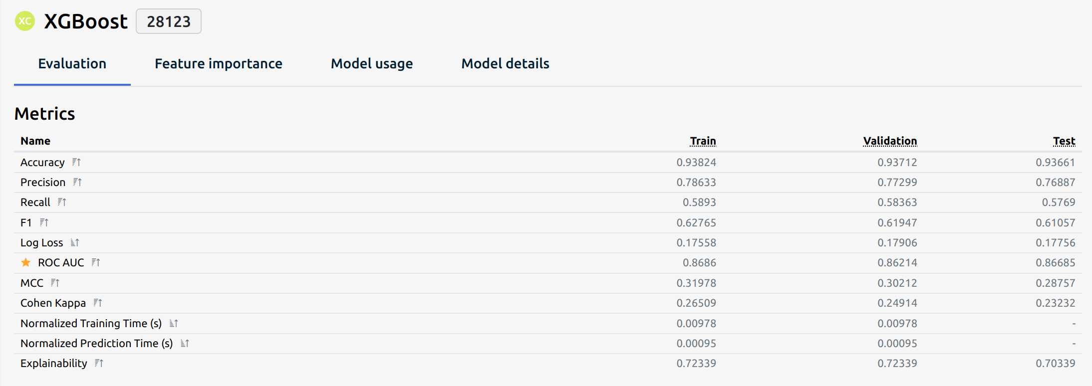
Classification Metrics
Classification metrics evaluate the performance of a classification model. The following metrics provide different insights depending on the model's use case and data characteristics.
Each classification metric provides different insights into a model’s performance. Selecting the right metric depends on the problem's specifics, such as class distribution, the cost of false positives or false negatives, and model efficiency requirements.
Each classification model is evaluated using these metrics:
1. Accuracy
Definition: Accuracy measures the proportion of correctly classified instances among all predictions.
Use Case: Useful when class distribution is balanced but can be misleading for imbalanced datasets.
2. Precision (Positive Predictive Value)
Definition: Precision measures the proportion of true positive predictions among all positive predictions.
Use Case: Important when false positives are costly, such as in medical diagnostics or fraud detection.
Note:
Precision answers the question: What proportion of predicted positives are actual positives?
3. Recall (Sensitivity or True Positive Rate)
Definition: Recall measures how many actual positive instances are correctly predicted.
Use Case: Crucial when missing positive cases is costly, such as in disease detection or spam filtering.
Note:
Recall answers the question: What proportion of actual positives were identified correctly?
4. F1 Score
Definition: The F1 score is the harmonic mean of Precision and Recall, balancing both metrics.
Use Case: Useful for imbalanced datasets where both precision and recall are important.
5. Log Loss (Logarithmic Loss)
Definition: Log Loss measures the uncertainty of predictions by penalizing false classifications with confidence. Lower values indicate better performance.
Where ( y_i ) is the actual label (0 or 1), ( p_i ) is the predicted probability for class 1, and ( N ) is the number of samples.
Use Case: Preferred in probabilistic models where prediction confidence matters.
6. ROC AUC (Receiver Operating Characteristic - Area Under Curve)
Definition: Measures the ability of a model to distinguish between classes. The AUC (Area Under Curve) ranges from 0 to 1, with higher values indicating better separation.
Use Case: Useful for evaluating binary classifiers, especially when dealing with imbalanced datasets.
7. Matthews Correlation Coefficient (MCC)
Definition: MCC is a balanced measure of correlation between actual and predicted classifications, even in imbalanced datasets.
Use Case: More reliable than accuracy for imbalanced datasets.
8. Cohen’s Kappa
Definition: Measures agreement between predicted and actual classifications while accounting for random chance.
Where ( P_o ) is the observed agreement and ( P_e ) is the expected agreement.
Use Case: Suitable for evaluating inter-rater reliability and classification performance.
9. Normalized Training Time
Definition: Measures the time taken to train a model, normalized for comparison across different models.
Use Case: Helps assess model complexity and computational efficiency.
10. Normalized Prediction Time
Definition: Measures the time taken to make predictions, normalized for comparison.
Use Case: Important for real-time applications where low latency is crucial.
11. Explainability
Definition: The degree to which a model’s predictions can be understood by humans. It can be qualitative or measured through techniques such as:
Methods of Explainability:
- Feature Importance: Identifying which features most influence predictions.
- Partial Dependence Plots (PDPs): Visualizing the relationship between features and predictions.
- LIME (Local Interpretable Model-agnostic Explanations): Explains individual predictions by approximating the model locally.
- SHAP (SHapley Additive exPlanations):
Use Case: Vital in high-stakes applications like healthcare, finance, and law enforcement.